Overview

#

In this project, I implemented a cloth simulation system, including collision handling and shader-based rendering. The work is divided into five main parts:

• Part 1: Masses and Springs
  I represent the cloth as a grid of point masses connected by springs. The springs enforce structural, shearing, and bending constraints, allowing the cloth to behave in a physically plausible way.

• Part 2: Simulation via Numerical Integration
  At each timestep, forces acting on the point masses—including internal spring forces and external forces like gravity—are computed. We use Verlet integration to update the positions of the masses, incorporating damping to simulate energy loss.

• Part 3: Handling Collisions with Other Objects
  I implement collision handling between the cloth and external objects, including spheres and planes. Collisions are detected and resolved by computing tangent points and applying friction-aware position corrections.

• Part 4: Handling Self-Collisions
  To efficiently handle collisions between different parts of the cloth itself, with spatial hashing to reduce the number of pairwise checks. Correction vectors are computed and averaged to separate overlapping point masses.

• Part 5: Shaders
  I explore visual rendering techniques using GLSL shaders. This includes implementing the Blinn-Phong lighting model, bump mapping, displacement mapping, and environment reflections via cubemaps. These techniques are combined in a custom shader to achieve enhanced visual realism.

Part 1: Masses and Springs

#

Spring Constraints

#

The model we use to simulate cloth is a system of point masses and springs. A set of uniformly distributed point masses are connected to their neighbors via springs. The springs impose three types of constraints that enable the point masses to behave like real cloth. These constraints are: structural constraints, shearing constraints, and bending constraints.

• Structural constraints connect each point mass to the one directly to its left and the one directly above it.
• Shearing constraints connect each point mass to its upper-left and upper-right diagonal neighbors.
• Bending constraints connect each point mass to the two point masses two points away in the left and upward directions.

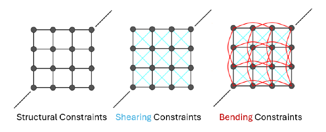
As illustrated in the figure, these different types of constraints help maintain the cloth’s good form structure and realistic deformation.

Results Gallery

#

Below is a visualization of the cloth wireframe with/without the three types of constraints.

Part 2: Simulation via Numerical Integration

#

Verlet Integration and Constraint Enforcement

#

At each simulation timestep, we compute the new position of every point mass. This begins with analyzing the forces acting on each point mass in order to determine its acceleration.

The total force on a point mass consists of two components: external forces and internal forces. External forces (such as gravity) are uniformly applied to all point masses. Internal forces originate from the springs and are computed using Hooke’s Law:
$$ \mathbf{F}_s = k_s \cdot (|\mathbf{p}_a - \mathbf{p}_b| - l) $$

where \( k_s \) is the spring constant, \(\mathbf{p}_a\) and \( \mathbf{p}_b \) are the positions of the two endpoints of the spring, and \( l \) is the spring’s rest length.

Once the total force is computed, we obtain the acceleration using Newton’s second law:
$$ \mathbf{a} = \frac{\mathbf{F}}{m} $$

To update the position of each point mass, we use Verlet integration:

$$ x_{t+\Delta t} = x_t + (1 - d)( x_{t} - x_{t - \Delta t} ) + \mathbf{a}_t \cdot \Delta t^2 $$

Here, \((x_t - x_{t - \Delta t})\) is used as an approximation of the velocity term, and \(d\) is the damping factor that models energy loss over time.

After computing the new positions, we enforce a constraint to prevent excessive deformation of the springs. Specifically, we ensure that no spring stretches more than a factor of \(\tau\) beyond its rest length. In my implementation, \(\tau = 0.1\). This is done by preserving the direction vector between the two endpoints of the spring and moving two endpoints inward to center accordingly making the spring length equals to \((1+\tau)\cdot l\)

Results and Experiments

#

In this section, we experiment with different values of key simulation parameters, including the spring constant \(k_s\), point mass density, and damping factor \(d\). We analyze how each of these parameters affects the behavior of the simulated cloth.

Spring Constant (\(k_s\))

#

The spring constant controls the internal elastic forces within the cloth. When \(k_s\) is set to a very low value, the cloth appears to have little to no elasticity, resulting in large deformations. As \(k_s\) increases, the cloth becomes stiffer and more resistant to deformation, exhibiting more elastic. However, if \(k_s\) is set too high, the internal forces become excessively large, causing the cloth to behave like jittering instead of falling naturally.

Density

#

Density will affect the mass of each point mass in the cloth and affect the relative influence of internal. Recalling the acceleration formula:

\[ \mathbf{a} = \frac{\mathbf{F}}{m} = \mathbf{a}_{\text{external}} + \frac{\mathbf{F}_s}{m} \]

In our implementation, the external acceleration (e.g., gravity) is directly applied as a constant, independent of mass. Therefore, changes in density do not affect the contribution of external forces to acceleration. However, increasing the density (and thus mass) reduces the contribution of spring forces to the overall acceleration.

From the visualization, we observe that cloth with low density exhibits less deformation and appears more elastic. In contrast, cloth with high density deforms significantly, similar to the behavior observed when using a low \(k_s\). This confirms that with higher mass, the effect of internal spring forces decreases.

Damping Factor ((d))

#

The damping factor reduces the energy from both internal and external forces. When the damping factor is set to a high value, the motion of the cloth slows down significantly. In particular, the descent of the cloth under gravity becomes noticeably slow, as the damping term suppresses the acceleration and velocity from all forces.

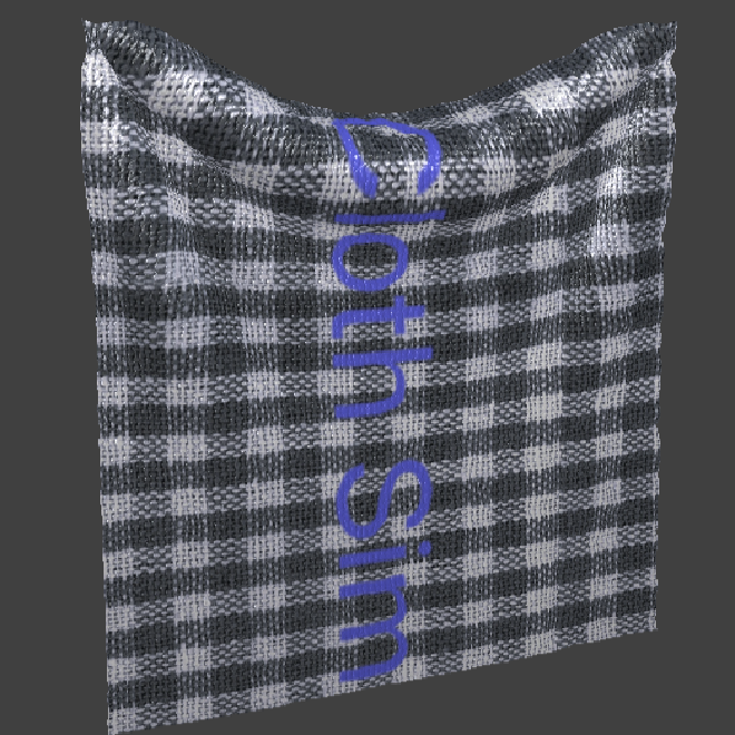
Finally, below is the shaded cloth from pinned4.json using default simulation parameters.

Part 3: Handling Collisions with Other Objects

#

In this part, I implement collision handling between the cloth and external objects, specifically spheres and planes. Collision resolution involves two steps: determining the tangent point where the correction should occur and updating the position while taking friction into account.

Collision Implementation

#

Sphere Collision

#

To detect collision with a sphere, we compute the direction vector:

$$ \mathbf{d} = \mathbf{p}_t - \mathbf{o} $$

where \(\mathbf{p}_t\) is the current position of the point mass, and \(\mathbf{o}\) is the center of the sphere. If \(|\mathbf{d}| < r\), where \(r\) is the radius of the sphere, the point mass is inside the sphere and a collision is detected.

To resolve the collision, we compute the tangent point by projecting the point outward along the direction vector to the sphere’s surface:

$$ \mathbf{p}_c = \mathbf{o} + r \cdot \frac{\mathbf{d}}{\|\mathbf{d}\|} $$

We then calculate the correction vector using the previous position \(p_{t-1}\):

$$ c = p_c - p_{t-1} $$

Taking friction \(f\) into account, we update the position of the point mass as:

$$ p_t’ = p_{t-1} + (1 - f)c $$

Plane Collision

#

To detect whether a point mass has passed through a plane, we consider a known point \(\mathbf{o}\) on the plane and the plane’s normal vector \(\mathbf{n}\). Define:

$$ v_1 = p_t - o, \quad v_2 = p_{t-1} - o $$

We compute the dot products \((\mathbf{v}_1 \cdot \mathbf{n})\) and \((\mathbf{v}_2 \cdot \mathbf{n})\). If their product is negative, the point mass has crossed the plane (i.e., the two positions lie on opposite sides of the plane), and a collision is detected.

To compute the tangent point, we parameterize the point mass’s trajectory:

$$ p = p_{t-1} + \alpha (p_t - p_{t-1}) $$

For this point to lie on the plane, it must satisfy:

$$ (p - o) \cdot n = 0 $$

Solving for \(\alpha\), we get:

$$ \alpha = \frac{(o - p_{t-1}) \cdot n}{(p_t - p_{t-1}) \cdot n} $$

Substitute back to find the tangent point:

$$ p_c = p_{t-1} + \alpha (p_t - p_{t-1}) $$

To avoid numerical artifacts and ensure the point lies slightly outside the surface, we offset the tangent point slightly in the direction along the normal and same side as the previous position:

$$ p_c = p_c \pm \text{SURFACE\_OFFSET} \cdot n $$

Add or subtract the offset based on the sign of \((\mathbf{p}_{t-1} - \mathbf{o}) \cdot \mathbf{n}\).

Finally, we apply the same position correction as in the sphere collision case:

$$ c = p_c - p_{t-1}, \quad p_t’ = p_{t-1} + (1 - f)c $$

Results

#

Here are scenes showing the cloth interacting with the sphere and plane. The cloth is set with \(k_s = 500, 5000, 50000\) respectively. The larger the spring constant, the cloth appears stiffer and more elastic, exhibiting less sagging upon collision with the sphere.

Part 4: Handling Self-Collisions

#

In this part, I implemented self-collisions within the cloth. To improve computational efficiency, I employ a spatial hashing technique. By dividing the space into discrete 3D boxes, we only consider potential collisions between point masses that fall within the same spatial box.

Spatial Hashing

#

Constructing the Spatial Hash

#

We define the bounding box of the cloth’s space as \((w_c, h_c, t_c)\), where \(w_c\) and \(h_c\) are the initial width and height of the cloth, and \(t_c = \max(w_c, h_c)\). This space is divided into 3D cells with shape:

$$ w = \frac{3w_c}{n_w}, \quad h = \frac{3h_c}{n_h}, \quad t = \max(w, h) $$

Here, \(n_w\) and \(n_h\) are the number of point masses along the width and height of the cloth, respectively. And the constant 3 here is an empirically chosen value to improve the performance of the spatial hashing. For each point mass, we compute its 3D box indices \((b_x, b_y, b_z)\):

$$ b_x = \left\lfloor \frac{p_x}{w} \right\rfloor, \quad b_y = \left\lfloor \frac{p_y}{h} \right\rfloor, \quad b_z = \left\lfloor \frac{p_z}{t} \right\rfloor $$

Then, we use a simple multiplicative hash function to compute a unique hash value:

$$ \text{hash} = b_x \cdot 149 + b_y \cdot 137 + b_z \cdot 163 $$

Here, 149, 137, and 163 are prime numbers chosen to reduce hash collisions. Each unique hash value corresponds to a distinct 3D box, and the hash table maps each box to a list of point masses it contains.

Collision Detection

#

For each point mass, we compute its hash and retrieve the list of other point masses in the same spatial box. We then iterate through this list and check for potential collisions. If another point mass (p_i) is found such that:

$$ \|\mathbf{p} - \mathbf{p}_i\| \leq 2 \cdot \text{thickness} $$

(where thickness is a threshold parameter), a self-collision is detected. For each such case, we compute a correction vector:

$$ \mathbf{c}_i = \frac{\mathbf{p} - \mathbf{p}_i}{|\mathbf{p} - \mathbf{p}_i|} \cdot (2 \cdot \text{thickness} - \|\mathbf{p} - \mathbf{p}_i\|) $$

This vector moves \(\mathbf{p}\) away from \(\mathbf{p}_i\) just enough to satisfy the minimum separation constraint.

After checking all neighbors, we compute the average of all correction vectors and scale it down by the number of simulation steps to avoid sudden large corrections:

$$ c_{\text{avg}} = \frac{1}{\text{simulation steps}} \cdot \frac{1}{N} \sum_{i=1}^N c_i $$

\(N\) here is not the number of points in the box, but the number of correction vectors computed. Finally, we apply the correction:

$$ \mathbf{p} = \mathbf{p} + \mathbf{c}_{\text{avg}} $$

Results

#

Here are the results of the self-collision detection and resolution. The cloth is set with \(k_s = 5000\) and density \(=15\).

And I observed the effect of varying the spring constant \(k_s\) and the density of the cloth. When \(k_s\) is small or the density is high, the cloth tends to form more wrinkles and experiences greater compression. In contrast, when \(k_s\) is large or the density is low, the cloth exhibits fewer wrinkles, and the regions of bending have a noticeably larger radius of curvature.

Part 5: Shaders

#

In this part, I use GLSL to implement some simple shaders to render the cloth.

How Shaders Work

#

Shaders are programs executed on the GPU to control how vertices and fragments are processed and rendered. In GLSL, a typical shader program consists of two main stages:

• Vertex Shader: Processes each vertex of the model. It transforms vertex positions, computes normals, texture coordinates, and other per-vertex data to be passed down the pipeline.
• Fragment Shader: Operates on each fragment generated from rasterizing primitives. It determines the final color of each pixel by combining lighting, texture, and material properties based on the structural data like position, normal, tangent, etc. passed from the vertex shader.

Together, vertex and fragment shaders enable the flexible control of the rendering, and efficiently utilize the parallel processing capabilities of GPUs.

Blinn-Phong Shading

#

The Blinn-Phong model is a simplified, empirical lighting model designed to approximate real-world light interaction. It has three main components: ambient, diffuse, and specular reflection.

• Ambient Lighting: Simulates the global illumination of the scene. It is approximated as a constant added to every fragment to represent indirect light:

  $$ k_a \cdot I_a $$ where \(k_a\) is the custom parameter and \(I_a\) is the ambient light intensity.

• Diffuse Lighting: Models how surfaces facing the light appear brighter, and those facing away appear darker, with a smooth transition in between. Given a light source with radiant intensity \(I\), the intensity at a distance \(r\) is:

  $$ \frac{I}{r^2} $$ According to Lambert’s cosine law, the amount of light reaching a surface depends on the angle between the light direction and the surface normal:
  $$ \cos\theta = \mathbf{l} \cdot \mathbf{n} $$

  where \(\mathbf{l}\) is the normalized direction from the fragment to the light source and \(\mathbf{n}\) is the surface normal. If \(\cos\theta < 0\), the light is behind the surface and contributes nothing. The full diffuse term is thus:

  $$ k_d \cdot \frac{I}{r^2} \cdot \max(0, \mathbf{n} \cdot \mathbf{l}) $$

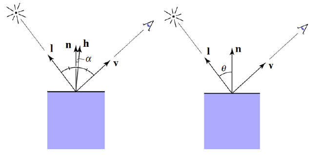
• Specular Highlight: Simulate shiny reflections on the surface. In the Blinn-Phong model, the specular term is computed using the half-vector \(\mathbf{h}\), defined as the normalized sum of the view direction \(\mathbf{v}\) and the light direction \(\mathbf{l}\):
  $$ \mathbf{h} = \frac{\mathbf{v} + \mathbf{l}}{|\mathbf{v} + \mathbf{l}|} $$

  The alignment between \(\mathbf{h}\) and the normal \(\mathbf{n}\) determines the intensity of the specular highlight:
  $$ k_s \cdot \frac{I}{r^2} \cdot \max(0, \mathbf{n} \cdot \mathbf{h})^p $$ where \(p\) is the shininess exponent. A larger \(p\) produces a narrower, sharper highlight, simulating a smoother surface.

Combining all three components, the complete Blinn-Phong reflection model becomes:
$$ \text{Color} = k_a I_a + k_d \frac{I}{r^2} \max(0, \mathbf{n} \cdot \mathbf{l}) + k_s \frac{I}{r^2} \max(0, \mathbf{n} \cdot \mathbf{h})^p $$

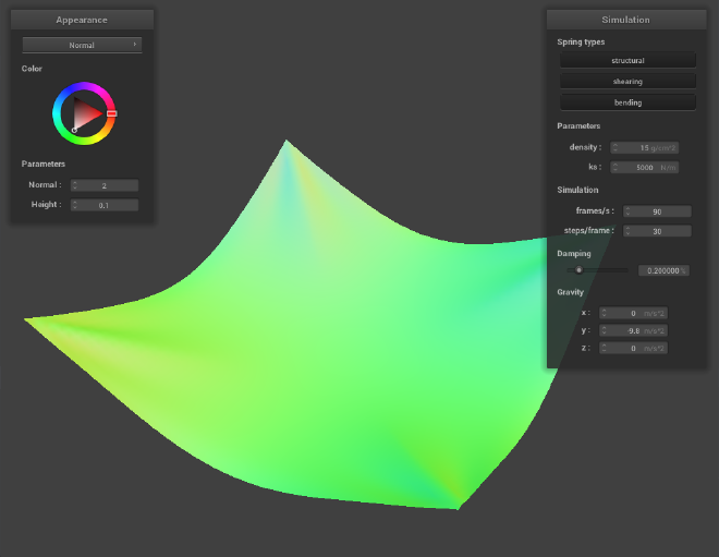
Here are the results using Blinn-Phong shading:

Results

#

Texture Mapping

#

Bump Mapping and Displacement Mapping

#

Here I use this rock wall texture, to compare the bump mapping and displacement mapping.

From the rendered results, it is evident that bump mapping creates the illusion of a bumpy or uneven surface by changing the surface normals used in lighting calculations. However, the underlying geometry remains unchanged—the positions of the vertices are exactly the same as in the original mesh. This technique is efficient and visually effective for simulating surface detail without increasing the polygon count.

In contrast, displacement mapping actually modifies the geometry of the object by displacing vertex positions based on a height or displacement map. This results in real changes to the mesh geometry, allowing for true geometric surface variation. As a result, displacement mapping can produce more realistic silhouettes and depth effects.

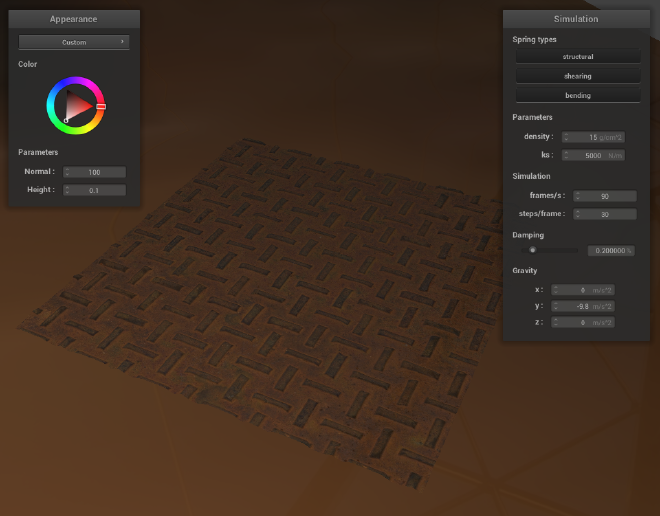
To further evaluate the effects of bump mapping and displacement mapping, we used a high-frequency roof texture and compared their behavior under varying levels of sphere mesh resolution. From the rendered results, we observe that the coarseness of the sphere mesh has little impact on bump mapping, but has a significant effect on displacement mapping.

This is because bump mapping only changes normals and does not rely on actual geometric detail. In contrast, displacement mapping modifies the vertex positions directly according to the height map. When the mesh resolution is low, i.e., when the sphere is coarse, there are too few vertices to accurately capture the height variations in the texture. This results in a form of ‘undersampling’, where fine features such as the depth between roof tiles are lost.

As shown in the rendered images, at a resolution of 16 (with -o 16 -a 16), the areas that should appear recessed between the tiles remain flat, failing to convey the intended depth. In contrast, a higher-resolution sphere more accurately reproduces the expected concavities and convexities of the roof surface.

Mirror Shader

#

Custom Shader

#

In this section, I combined several previously implemented shaders to achieve improved visual quality. The enhancements primarily involve two key additions: texturing the displacement shader and using a cubemap for environment lighting.

First, I modified the displacement shader to incorporate texture-based surface color. Specifically, the texture color is used as the albedo term \(I_t\) in the Blinn-Phong shading model. The lighting components were updated as follows:

$$ \text{Ambient} = K_a \cdot I_a \cdot I_t $$ $$ \text{Diffuse} = K_d \cdot \frac{I}{r^2} \cdot \max(0, \mathbf{n} \cdot \mathbf{l}) \cdot I_t $$ This allows the surface color to be determined by the texture, giving a more realistic appearance when combined with geometric displacement. Next, I integrated environment reflections using a cubemap. Building upon the mirror shader, introduced a reflectivity parameter to blend between the original Blinn-Phong shading result and the reflection sampled from the cubemap. The final fragment color is computed using linear interpolation:

$$ \text{FinalColor} = (1 - \text{reflectivity}) \cdot \text{BlinnPhongColor} + \text{reflectivity} \cdot \text{CubemapReflection} $$

This produces a realistic material effect where surfaces exhibit both texture-based shading and environment-based reflections, with the balance controlled by the reflectivity parameter.