
Overview#
In this project, I implemented a physically-based renderer using the path tracing algorithm, achieving realistic rendering effects. The implementation consists of five main components:
Ray Generation and Primitive Intersection
I implemented ray generation from each pixel, transforming screen coordinates into world space, using the Möller–Trumbore Algorithm for efficient triangle intersection detection.Bounding Volume Hierarchy (BVH) Acceleration
Constructed a BVH tree to hierarchically partition scene primitives, improving intersection tests. Implemented different BVH splitting heuristics and compared their performance.Direct Illumination
Calculated direct lighting by estimating radiance contributions from light sources. Used hemisphere sampling to determine one-bounce light radiance contributions and improved efficiency with importance sampling.Global Illumination
Extended direct illumination to handle multiple bounces, simulating indirect lighting effects. Implemented recursive radiance computation to handle indirect illumination and used Russian Roulette termination to maintain an unbiased estimate while reducing excessive computation.Adaptive Sampling
Introduced an adaptive sampling method to dynamically adjust the number of samples per pixel. Tracked variance and confidence intervals to terminate sampling early for converged pixels. Significantly improved rendering efficiency by allocating more samples to noisy regions while reducing computation in smooth areas.
Part 1: Ray Generation and Scene Intersection#
Ray Generation and Primitive Intersection Overview#
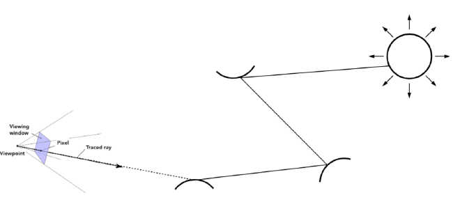
Ray tracing is a rendering technique that enables the simulation of highly realistic physical effects. The fundamental idea involves casting rays from each pixel on the screen (the camera plane) outward and determining whether these rays intersect with any objects in the scene, specifically whether they intersect with geometric primitives such as triangles or spheres. The color of a pixel is then determined based on the color of the object the ray intersects. This method effectively simulates the propagation of light, providing good space for enhancement to achieve more photorealistic rendering. In subsequent sections, I will incorporate additional factors, such as the material properties and light reflection, to further enhance realism in rendering.
Ray Generation#
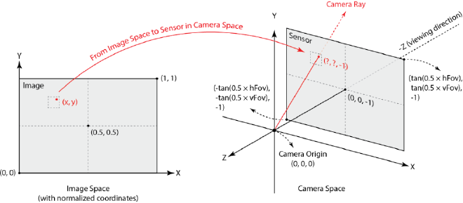
For each pixel on the screen, multiple sub-pixel positions are sampled to generate multiple rays. These rays collectively determine the final pixel color. The first step is to transform the sampled screen coordinates into the camera coordinate system. This transformation begins with normalizing the screen coordinates:
$$ x’ = \frac{x}{\text{screen width}}, \quad y’ = \frac{y}{\text{screen height}} $$
Next, the left-bottom and right-top corners of the camera plane are computed as:
$$
p_{\text{left bottom}} = (-\tan(\text{hFov}/2), -\tan(\text{vFov}/2), -1)
$$
$$
p_{\text{right top}} = (\tan(\text{hFov}/2), \tan(\text{vFov}/2), -1)
$$
where \( \text{hFov} \) and \( \text{vFov} \) are the horizontal and vertical fields of view, respectively. Here we put camera plane at \(z=-1\) plane. The normalized coordinates are then used for interpolation to obtain the corresponding position in the camera space:
\[
x_{\text{ray}} = (1-x’)x_{\text{left bottom}} + x’x_{\text{right top}}
\]
\[
y_{\text{ray}} = (1-y’)y_{\text{left bottom}} + y’y_{\text{right top}}
\]
\[
z_{\text{ray}}=-1
\]
This method provides flexibility in handling cameras with varying aspect ratios and fields of view (FOV).
Once the position in the camera coordinate system \(p_{\text{ray}} = (x_{\text{ray}}, y_{\text{ray}},z_{\text{ray}}) \) determined, it can be transformed into world coordinates \(P_{\text{ray}}\). With the known camera origin \(O\), the ray direction is computed as the difference between the world-space position and the camera origin: \(D = P_{\text{ray}} - O\). The ray is given by: \(P = O + tD\)
Primitive Intersection#
In this project, rays may intersect with two types of primitives: triangles and spheres.
Triangle Intersection#
To determine whether a ray intersects with a triangle, we use the Möller–Trumbore algorithm. Any point lying on a triangle can be expressed in barycentric coordinates as:
\[ P = \alpha P_1 + \beta P_2 + \gamma P_3, \quad \text{where} \quad \alpha + \beta + \gamma = 1 \]
Since the intersection point \( P \) lies on the ray, we substitute \( P = O + tD \). This leads to:
\[ O + tD = (1 - \beta - \gamma) P_1 + \beta P_2 + \gamma P_3 \]
Expanding:
\[ O + tD = P_1 + \beta (P_2 - P_1) + \gamma (P_3 - P_1) \] \[ O - P_1 = -tD + \beta (P_2 - P_1) + \gamma (P_3 - P_1) \]
This can be rewritten in matrix form:
\[ O - P_1 = [-D, P_2 - P_1, P_3 - P_1] \begin{bmatrix} t \\ \beta\\ \gamma \end{bmatrix} \]
This is the same as \( Ax = b \), where:\( A = [-D, P_2 - P_1, P_3 - P_1] \), \( x = [t, \beta, \gamma]^T \), \( b = O - P_1 \). Using Cramer’s Rule, we solve for \( x \) using determinants:
\[ [t, \beta, \gamma] = \frac{1}{|A|} \begin{bmatrix} |A_1| \\ |A_2| \\ |A_3| \end{bmatrix} \]
Where \( A_i \) is matrix \( A \) with the \( i \)-th column replaced by \( b \). This simplifies to:
\[ = \frac{1}{S_1 \cdot E_1} \begin{bmatrix} S_2 \cdot E_2 \\ S_1 \cdot S \\ S_2 \cdot D \end{bmatrix} \]
Where:
- \( E_1 = P_2 - P_1 \)
- \( E_2 = P_3 - P_1 \)
- \( S = O - P_1 \)
- \( S_1 = D \times E_2 \)
- \( S_2 = S \times E_1 \)
We also use a trick to calculate the determinant of a \( 3 \times 3 \) matrix:
\[
|A,B,C| = -(A \times C)\cdot B = -(C \times B) \cdot A = -(B \times A) \cdot C
\]
After solving for \( t \), we check that it lies within the camera’s near and far clipping planes. Also, \( \beta, \gamma \in [0, 1] \), and \( \beta + \gamma \leq 1 \). If these conditions hold, the intersection is inside the triangle. And the only one special case is when the ray is parallel to the triangle, the \( S_1 \cdot E_1 = 0 \) will be zero, we can check this case ahead.
Sphere Intersection#
A point on the surface of a sphere satisfies the equation:
\[ (p - C)^2 - R^2 = 0 \]
Where \( C \) is the sphere’s center and \( R \) is its radius. Substituting the ray equation \( p = O + tD \):
\[ at^2 + bt + c = 0 \]
With:
- \( a = D \cdot D \)
- \( b = 2 (O - C) \cdot D \)
- \( c = (O - C) \cdot (O - C) - R^2 \)
Solving this gives:
\[ t = \frac{-b \pm \sqrt{b^2 - 4ac}}{2a} \] The nature of the solutions to this quadratic equation determines the intersection: If there are two real roots, the smaller positive root is selected as the intersection point; If there is one real root, the ray grazes the sphere tangentially; If there are no real roots, there is no intersection.
Results Gallery#
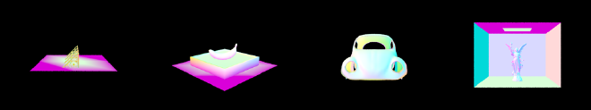
Here are some results with normal shading, after implementing ray casting and intersection tests:


Part 2: Bounding Volume Hierarchy#
Bounding Volume Hierarchy Overview#
To accelerate path tracing, we can store scene primitives using a Bounding Volume Hierarchy (BVH). BVH is a binary tree structure that recursively partitions the primitives into different bounding boxes. Primitives are stored in the leaf nodes, while internal nodes contain bounding boxes that enclose all primitives within their child nodes. This hierarchical structure eliminates the need to check all primitives for ray intersections. Instead, we first check whether the ray intersects with a bounding box. If there is no intersection, we can immediately discard the entire bounding box and all its contained primitives, significantly improving performance.
BVH Construction#
The BVH construction process is straightforward. We recursively create BVH nodes by computing the bounding box of all primitives within a node, then splitting them into two groups using a heuristic partitioning strategy. This process continues until the number of primitives in a node falls below a predefined threshold.
The key challenge in BVH construction is selecting an efficient partitioning heuristic to split primitives into two groups. In this project, I implemented these partitioning strategies:
- Median Element Splitting
- Average Position Splitting
Median Element Splitting#
The median splitting method selects a partitioning axis and divides primitives at the median element along that axis. First, identify the longest axis of the bounding box that encloses all primitives. This ensures the bounding boxes remain more cube-like rather than elongated, which reduces the likelihood of rays hitting bounding boxes unnecessarily. Sort the primitives along this axis. Then select the median element \(\frac{1}{2}\) as the splitting point. Assign the primitives smaller than the median to one group and larger than the median to the other. This method ensures that both child nodes contain a roughly equal number of primitives, but it may result in overlapping bounding boxes and empty spaces, which can impact traversal efficiency.
Average Position Splitting#
The average position splitting method is similar to median splitting, but instead of selecting the median element, it computes the average position of all primitives along the longest axis:
\[ \bar{p} = \frac{1}{N} \sum_{i=1}^{N} p_i \]
where \( p_i \) is the position of the \( i \)th primitive. This approach reduces the number of overlapping bounding boxes and empty space, potentially leading to better ray traversal performance. However, it does not guarantee that both groups contain an equal number of primitives, which can sometimes result in an unbalanced tree.
Comparisons of Splitting Methods#
To evaluate the effectiveness of these BVH partitioning methods, I rendered scenes with different splitting strategies. It is obvious that using BVH significantly reduces rendering time compared to no acceleration structure. The following table summarizes the rendering time for different scenes with a relatively small number of meshes. The resolution is \(800 \times 600\) and the number of threads is 8.
| Scene | Without BVH (s) | Median Element Splitting (s) | Average Position Splitting (s) |
|---|---|---|---|
| Building | 19.652 | 0.036 | 0.035 |
| Banana | 2.099 | 0.042 | 0.0362 |
| Beetle | 6.924 | 0.041 | 0.037 |
| CBlucy | 164.699 | 0.058 | 0.046 |
Results Gallery#
In this section I present rendering results for large .dae files, which can now be rendered efficiently using BVH acceleration.


Part 3: Direct Illumination#
Overview#
After implementing ray generation in Part 1, each pixel on the screen now emits multiple rays and detects intersections with objects. If a ray directly intersects with light source, the emission of the light source is returned, contributing directly to the brightness of the corresponding pixel. However, if the ray intersects a non-emissive object, a secondary reflected ray will be generated. Using the incident and outgoing rays, we compute radiance using the reflection equation.
Direct Illumination Calculation#
Given a ray originating from the screen:
\[
r = o + td
\]
If an intersection is detected at \( t’ \), the hit point is:
\[
p = o + t’d
\]
At \( p \), we see this ray as the outgoing ray \( r_{\text{out}} \) in direction \( w_o \). To estimate the incoming radiance at \( p \), we sample an incident ray \( r_{\text{in}} \) from the hemisphere above the surface in direction \( w_i \). The probability of sampling a given direction \( w_i \) uniformly over the hemisphere is:
\[
p(w_i) = \frac{1}{\Omega} = \frac{1}{\int_0^{2\pi} \int_0^{\pi/2} \sin\theta d\theta d\phi} = \frac{1}{2\pi}
\]
Using this sampled incoming ray (but oriented outward), we check whether it intersects a light source. If so, the light’s emission serves as the incoming radiance \( L_{\text{in}} \), which can be used in the reflection equation:
\[ L_{\text{out}} = \int_{H^2} f_r(p, w_i \to w_o) L_{\text{in}}(p, w_i) \cos\theta_i , dw_i \]
where:
- \( f_r(p, w_i \to w_o) \) is the bidirectional reflectance distribution function (BRDF), describing how light is reflected.
- \( L_{\text{in}}(p, w_i) \) is the incoming radiance from direction \( w_i \).
- \( \cos\theta_i \) accounts for the angle between the incident direction and the surface normal, computed as \( \cos\theta_i = w_i \cdot n \). Since we use a local coordinate system where \( n = (0,0,1) \), this simplifies to the z-component of \( w_i \).
Since Monte Carlo integration is used to estimate the integral, the equation transforms into:
\[ L_{\text{out}} = \frac{1}{N} \sum_{i=1}^{N} \frac{f_r(p, w_i \to w_o) L_{\text{in}}(p, w_i) \cos\theta_i}{p(w_i)} \]
where \( p(w_i) = 1 / 2\pi \), which was computed during sampling. By sampling \( N \) incident rays and applying this equation, we estimate the outgoing radiance, which determines the final pixel color.
Direct Lighting Using Importance Sampling#
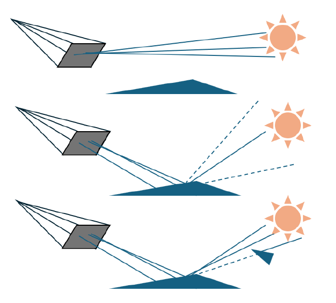
The uniform hemisphere sampling method has a major drawback: most sampled rays do not hit light sources, leading to inefficient convergence. To improve efficiency, importance sampling focuses only on sampling rays towards light sources, adjusting probabilities accordingly.
Instead of sampling random hemisphere directions, we directly sample a ray that originates from the hit point \( p \) and points toward a randomly chosen location on a light source. Here are key modifications:
Sampling Light Sources
Instead of uniform sampling, we directly sample a point on the light source and compute the corresponding direction \( w_i \). This ensures that the sampled ray contributes directly to the final radiance calculation.Handling Occlusion
Unlike uniform sampling, we need to check if the sampled ray is blocked before contributing radiance. When setting the maximum ray parameter \( t_{\max} \), we use a value slightly less than the actual distance between \( p \) and the light source. If any object intersects this ray before reaching the light, it means the light is blocked.Adjusting the Probability Distribution
The original uniform sampling probability was \( 1 / 2\pi \). In importance sampling, we use the actual probability distribution of selecting a point on the light source, replacing the uniform hemisphere probability.
Once these modifications are applied, the same Monte Carlo integration formula is used to compute the radiance.
Comparison of Uniform and Importance Sampling#
Using 16 samples per pixel and 8 samples per light source, here are the results of uniform and importance sampling for direct illumination. The importance sampling method significantly reduces noise. Meanwhile, if the scene only contains a point light, it is very hard to sample the light source uniformly, which will lead to a black image. Importance sampling solves this problem by directly sampling the light source.
Results are shown below:


Comparison of Different Number of Light Samples#
The number of light samples significantly impacts the quality of the rendered image. With more light samples, the soft shadows becomes less noisy and more accurate smooth. Here are the results of rendering the same scene with different numbers of light samples(1, 4, 16, 64):


Part 4: Global Illumination#
Overview#
In the previous section on Direct Illumination, we only considered rays that, after a single bounce, directly hit a light source. However, real-world illumination consists of multiple bounces, where light interacts with various surfaces before reaching the camera. To achieve global illumination, we must account for these indirect light contributions.
When a ray reflects off a surface at a point \( p_1 \), it can:
- Directly hit a light source (as handled in Direct Illumination).
- Hit another object, which itself may have received light from other sources.
Each surface’s material determines how light is reflected. After the first bounce, we sample a new direction \( w_i \) for the next ray, according to the material’s reflection properties. The probability density function of this sampling is denoted as \( p(w_i) \). This new ray is then traced through the scene to determine whether it intersects another object. If an intersection occurs at point \( p’ \), the exiting radiance from \( p’ \) contributes to the incident radiance at \( p_1 \), following the reflection equation and Monte Carlo integration.
\[ \begin{aligned} L_{out} &= \frac{1}{N} \sum_{i=1}^{N} \frac{f_r(p, w_i \to w_o) L_{in}(p, w_i) \cos\theta_i}{p(w_i)}\\ &= \frac{1}{N_1} \sum_{i=1}^{N_1} \frac{f_r(p, w_i \to w_o) L_{\text{in;light}}(p, w_i) \cos\theta_i}{p(w_i)} + \frac{1}{N_2} \sum_{j=1}^{N_2} \frac{f_r(p, w_j \to w_o) L_{\text{in;indirect}}(p, w_j) \cos\theta_j}{p(w_j)} \end{aligned} \]
Recursive Radiance Calculation#
Since every point in the scene receives light either directly from the source or indirectly via reflections, we recursively compute the radiance at each intersection point. And the radiance contribution diminishes with each bounce, ensuring convergence to a stable solution.
- At each bounce, the reflection equation is applied to determine how much light is transferred from the new intersection point to the previous one.
- The last bounce only considers direct illumination from light sources, make sure it has a value to back propagate to the previous bounce.
- Each bounce reduces radiance, since both the BRDF \( f_r \) and the cosine term \( \cos\theta_i \) are values between 0 and 1. After multiple bounces, the radiance contribution becomes super small, ensuring the rendering equation converges.
Stopping the Recursion#
Since recursive evaluation of all bounces would require infinite computation, we must decide when to terminate ray recursion. There are two approaches: Fixed Maximum Depth A straightforward approach is to limit the recursion depth to a predefined number of bounces. After this depth, the last bounce only considers direct illumination from light sources, ignoring additional reflections. It is simple and ensures termination but introduces bias, as the radiance contribution from uncalculated \(N+1\) bounces is ignored.
Russian Roulette Termination A more sophisticated approach is Russian Roulette, where each recursive bounce randomly decides whether to continue with probability \( p_{\text{rr}} \). If the recursion stops, no further contributions are added. At each bounce, continue with probability \( p_{\text{rr}} \), and terminate with probability \( 1 - p_{\text{rr}} \). To compensate for early termination, we adjust the computed radiance: \[ L_{\text{rr}} = \frac{L}{p_{\text{rr}}} = \frac{1}{N} \sum_{i=1}^{N} \frac{f_r(p, w_i \to w_o) L_{\text{in}}(p, w_i) \cos\theta_i}{p(w_i)p_{\text{rr}}} \quad \text{with probability } p_{\text{rr}} \] \[ L_{\text{rr}} = 0, \quad \text{with probability } 1 - p_{\text{rr}} \]
This ensures that the expected radiance remains unbiased: \[ E[L_{\text{rr}}] = p_{\text{rr}}E\left[\frac{L}{p_{\text{rr}}}\right] + (1 - p_{\text{rr}})E[0] = E[L] \]
Results#
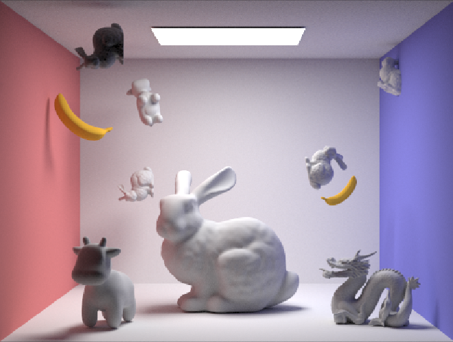
Here are some results, rendered with 1024 samples per pixel, 16 samples per light source, and 5 bounces, with maximum depth termination.


Comparison of Direct and Global Illumination#
Here are two images rendered with ONLY direct illumination or ONLY global illumination. The indirect illumination provides more realistic effects, for example, the color of wall will affect the color of the spheres, and like soft shadows and more accurate lighting. The direct illumination image appears flat and lacks the depth and realism of the global illumination result.


Comparison of Bounce Depth#
The number of bounces significantly impacts the quality of the rendered image. More bounce depth provides more realistic lighting effects, such as soft shadows and color bleeding. To analyze the progressive contribution of light bounces to global illumination, below are renderings of the same scene with different bounce depths (0, 1, 2, 3, 4, 5), where each image displays only the illumination from that specific bounce number rather than the cumulative radiance contribution from all bounces. Images are rendered with 1024 samples per pixel and 16 samples per light source.
For example, in 2-nd and 3-rd bounce, the light from the light source is reflected to the wall, and then the light from the wall is reflected to the bunny, making the left side of bunny red and the right side blue. It provides a more realistic effect, making light smoothly fuse in the scene.


Russian Roulette Results#
Here are results of rendering the same scene with Russian Roulette termination, I set termination probability to 0.3. Sample with 1024 samples per pixel, 16 samples per light source, and (0, 1, 2, 3, 4, 100) bounces.


Part 5: Adaptive Sampling#
In the previous section on Global Illumination, we required thousands of samples per pixel to reduce noise and produce high-quality images. However, many pixels—such as those on flat walls or uniformly lit surfaces—converge quickly, meaning additional samples do not significantly change their final color.
Adaptive sampling addresses this inefficiency by dynamically adjusting the number of samples per pixel. Instead of using a fixed sample count for all pixels, we stop sampling pixels that have already converged, allowing us to focus computational resources on noisy regions.
Statistical Basis for Adaptive Sampling#
To determine when a pixel has converged, we track the running statistics of its sampled radiance values. Specifically, for each pixel, we maintain:
- Sum of sample values:\(S_1 = S_1 + x_{\text{new}}\)
- Sum of squared sample values:\(S_2 = S_2 + x_{\text{new}}^2\) where \( x_{\text{new}} \) is the illuminance of a newly sampled ray.
After \( n \) samples, we compute:
\[ \mu = \frac{S_1}{n},\quad \sigma^2 = \frac{1}{n-1} \left( S_2 - \frac{S_1^2}{n} \right) \] Using these statistics, we define an uncertainty interval:
\[ I = 1.96 \frac{\sigma}{\sqrt{n}} \]
where \( I \) represents the 95% confidence interval—meaning that with 95% probability, the true pixel radiance lies within \( \mu - I \) and \( \mu + I \).
Stopping Criterion#
We define a threshold for convergence, using a user-defined tolerance maxTolerance:
\[
I \leq \text{maxTolerance} \times \mu
\]
If \( I \) is small relative to \( \mu \), we conclude that additional samples are unlikely to change the final pixel value significantly, and we stop sampling for that pixel. If \( I \) is large, it indicates high variance in the samples, meaning that the pixel is still noisy and requires more samples.
Results#
Using adaptive sampling, we observe that certain areas in the rendered images converge quickly and require fewer samples, while others need more samples to achieve a noise-free result. Here are the results of rendering the same scene with adaptive sampling, using 2048 samples per pixel, 1 sample per light source, and 5 bounces. maxTolerance is set to 0.05.


Observations on Sample Distribution#
Regions that Converge Quickly (Fewer Samples Required)#
Flat Surfaces. (e.g., walls, floors) These areas receive smooth, uniform illumination with little variation. Once a stable luminance value is reached, additional samples provide minimal improvements.
Surfaces Directly Facing the Light Source. (e.g., Wall-E’s front-facing panels, Bunny’s back) Since these surfaces receive strong, direct illumination, their brightness values stabilize quickly.
Regions that Require More Samples (High Sample Counts)#
Surfaces in Shadows. (e.g. The back of objects facing away from the light source, such as the foot area of the bunny) Indirect lighting relies on multiple bounces, leading to higher variance in radiance calculations.
Structurally Complex Regions. (e.g. Wall-E’s wheels and mechanical components) These areas contain fine details and varying surface orientations, increasing the likelihood of high variance in indirect lighting contributions.