Overview

#

In this project, I implemented Bézier Curves and Surfaces and explored Triangle Meshes, including various local transformations and mesh upsampling techniques. The following is a summary of each part:

Part 1: Bézier Curves with 1D de Casteljau Subdivision

#

In this section, I implemented 2D Bézier curves using the de Casteljau algorithm. By repeatedly applying linear interpolation (lerp), I was able to construct Bézier curves with an arbitrary number of control points. Additionally, I analyzed the working principle of the algorithm.

Part 2: Bézier Surfaces with Separable 1D de Casteljau

#

This section extends Bézier curves to Bézier surfaces, utilizing two parameters \( u, v \) to control surface generation through separable applications of the de Casteljau algorithm.

Part 3: Area-Weighted Vertex Normals

#

This section implements an approach to computing vertex normals using area-weighted averaging. Additionally, I compared Flat Shading and Phong Shading to analyze their differences in rendering smooth surfaces.

Part 4: Edge Flip

#

The first local transformation applied to meshes: edge flipping, which swaps the shared edge of two adjacent triangles.

Part 5: Edge Split

#

This section implements edge splitting, which introduces additional vertices and triangle faces, laying the foundation for mesh subdivision. Furthermore, I extended the implementation to handle boundary edge splitting.

Part 6: Mesh Subdivision

#

I implemented mesh subdivision. This section also discusses potential issues that arise in subdivision, particularly in preserving sharp corners and edges, and explores possible solutions.

---

Part 1: Bézier Curves with 1D de Casteljau Subdivision

#

Introduction to Bézier Curves

#

Bézier curves can be represented using the general algebraic formula:

$$ b^n(t) = \sum_{j=0}^{n} b_j B_j^n(t) $$

where \( b_j \) represents the coordinates of the control points, which can be values, points, or vectors. Since we are drawing curves in a 2D plane, these coordinates represent two-dimensional positions. \( B_j^n(t) \) refers to the Bernstein polynomials, which determine the interpolation scheme:

$$ B_j^n(t) = \binom{n}{j} t^j (1-t)^{n-j} $$

By replacing them with different functions of \( t \), we can obtain different types of curves, such as Catmull-Rom splines and Hermite interpolation. To get rid of mathematical computations, we use the Casteljau Algorithm, which derives points on the final curve through iterative interpolation between control points.

The Casteljau Algorithm

#

Given \( n+1 \) control points (defining a Bézier curve of degree \( n \)), we iteratively perform linear interpolation between adjacent points \( p_i \) and \( p_{i+1} \) using parameter \( t \):

$$ p_i^1 = (1-t) p_i + t p_{i+1} $$

This produces \( n \) new intermediate control points. We then repeat the interpolation process with these \( n \) new points to generate \( n-1 \) control points. This process continues until only a single point remains, which represents the point on the Bézier curve corresponding to the parameter \( t \).

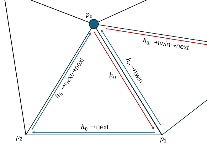
The Casteljau algorithm effectively constructs a coefficient pyramid using repeated interpolation with \( t \), as illustrated in the figure. The final point at the top of the pyramid is computed by recursively combining the original \( n+1 \) control points through multiplications with \( t \) and \( (1-t) \). This hierarchical structure aligns with the Bernstein polynomial formulation.

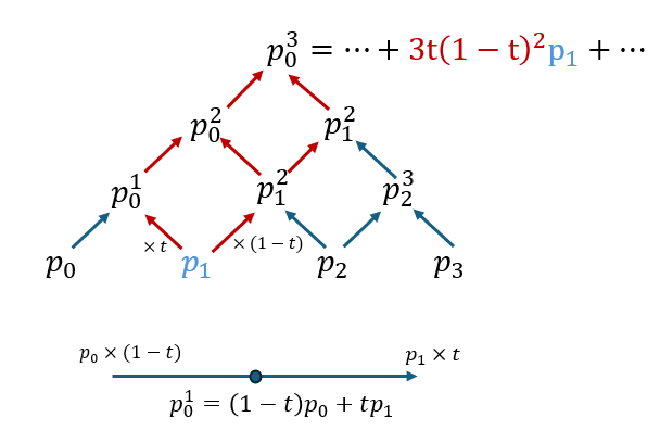
For example, as shown by the red arrows in the figure, the contribution of \( p_1 \) to the final curve point \( p_0^3 \) is determined by the interpolation process. A rightward arrow corresponds to multiplication by \( (1-t) \), while a leftward arrow corresponds to multiplication by \( t \). Since there are three distinct paths from \( p_1 \) to the final point, each path involving two rightward moves and one leftward move, the overall contribution of \( p_1 \) is \( 3t(1-t)^2 \), which precisely matches the Bernstein polynomial \( B_1^3(t) = \binom{3}{1} t (1-t)^2 = 3t(1-t)^2 \).

This is the fundamental principle behind how the Casteljau algorithm evaluates Bézier curves.

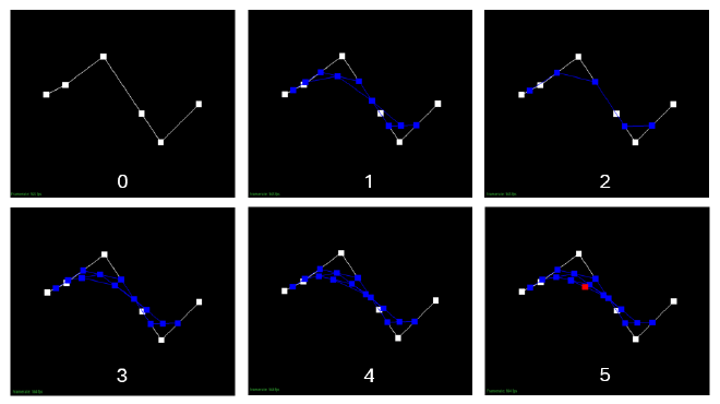
Result Gallery

#

Below is a Bézier curve of degree 5, with 6 control points. The interpolation process requires 5 levels of interpolation. The images below illustrate the step-by-step process leading to the final curve point.

Full Curve and Different Curves

---

Part 2: Bézier Surfaces with Separable 1D de Casteljau

#

Extending Bézier curves to Bézier surfaces is straightforward—we simply introduce more control points and additional parameters \((u, v)\).

For example, given a \( m \times n \) grid of control points, we begin by processing each row separately. Each row consists of \( n \) control points, and for each row, we construct a Bézier curve using the parameter \( u \). This results in \( m \) intermediate Bézier curve points when \( u \) is fixed.

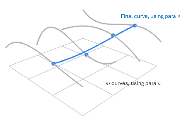
Next, we treat these \( m \) intermediate points as control points and construct another Bézier curve using parameter \( v \). The result of this second interpolation gives a single point on the Bézier surface at \((u, v)\).

This approach effectively extends the de Casteljau algorithm from 1D Bézier curve interpolation to a separable 2D interpolation scheme, allowing us to generate smooth Bézier surfaces efficiently.

---

Part 3: Area-Weighted Vertex Normals

#

In shading computations, normals play a crucial role, as they are essential for lighting calculations, including specular reflection, diffuse shading, ray tracing… If we use per-triangle normals directly—also known as flat shading—the surface will appear exactly super faceted. This is because each triangle has a single normal, and the entire region covered by that triangle will be shaded as a flat plane, defined by this one normal.

To achieve a smoother appearance, we use vertex normals, which are computed as interpolated values from the normals of surrounding triangles. This technique allows for smoother transitions between adjacent triangles, creating a more visually appealing surface.

Implementation Details

#

Given a vertex, we begin by retrieving a halfedge \( h_0 \) that originates from this vertex. This halfedge belongs to a triangle, we can use it to access the triangle’s geometry.

1. Compute Triangle Normals with Area Weighting. Using the halfedge traversal, we identify the three vertices of the triangle, denoted as \( p_0, p_1, p_2 \). Compute two edge vectors: $$ v_1 = p_1 - p_0, \quad v_2 = p_2 - p_1 $$ Compute the normal of the triangle using the cross product: $$ n = \frac{v_1 \times v_2}{|v_1 \times v_2|} $$ And the magnitude of \( v_1 \times v_2 \) divided by 2 gives the area of the triangle. $$ A = \frac{1}{2} |v_1 \times v_2| $$ Multiply the normal \(n\) by the area \(A\) to obtain the weighted normal for the triangle.

2. Accumulate Weighted Normals from Neighboring Triangles. To process the next triangle sharing the vertex, we follow the halfedge structure: Use \( h_0 \)’s twin halfedge to move to the neighboring triangle. From the twin, access the next halfedge, which starts at the same vertex. $$ h_{i+1} = h_i \to \text{twin} \to \text{next} $$ Repeat the normal computation for this triangle. Continue the traversal using \( h \to \text{twin} \to \text{next} \) until returning to the original halfedge \( h_0 \), ensuring all incident triangles have been visited.

3. Compute Final Vertex Normal. Sum all area-weighted normals obtained from the neighboring triangles. Normalize the final vector to obtain the vertex normal. $$ \sum_{i=0} \frac{A_i \cdot n_i }{|A_i \cdot n_i|} $$

   

By weighting the normals based on the triangle areas, this method ensures that larger triangles contribute more significantly to the vertex normal computation, resulting in a more accurate and visually smooth shading effect.

Result Gallery

#

The left column shows the original flat shading, while the right column displays the smooth shading effect achieved using area-weighted vertex normals (Phong shading).

Flat shading vs. Phong shading

---

Part 4: Edge Flip

#

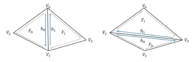
Flipping an edge in a manifold mesh involves replacing an existing edge with a new one that connects the two previously unconnected vertices. Since the input mesh is guaranteed to be manifold, each edge (except for boundary edges) is shared by exactly two triangles. The edge flip operation replaces the original edge, which connects \( V_0 \) and \( V_1 \), with a new edge connecting \( V_2 \) and \( V_3 \).

Implementation Details

#

1. Edge Selection. Before proceeding, we check whether the selected edge lies on the boundary. If either of its two adjacent triangles is a boundary face, we skip the operation, as a flip would be invalid in such cases.

2. Identifying Key Elements.

• Retrieve the halfedge \( h_0 \) stored in the edge to be flipped and define its root vertex as \( V_0 \).
• Get \( h_0 \)’s twin halfedge \( h_1 \), and define its root vertex as \( V_1 \).
• The remaining two vertices, \( V_2 \) and \( V_3 \), can be accessed by following two consecutive next pointers from \( h_0 \) and \( h_1 \), respectively.

3. Flipping the Edge.

• The key operation is updating the vertices associated with \( h_0 \) and \( h_1 \): $$ h_0 \rightarrow \text{vertex} = V_2, \quad h_1 \rightarrow \text{vertex} = V_3 $$ The reason it’s important to make the vertex of \(h_0\) \(V2\) instead of \(V3\) here is that by flipping the edge this way, the halfedge within a triangle stays in the same direction as the original (clockwise or counterclockwise)
• This effectively change the edge to connect \( V_2 \) and \( V_3 \).

4. Pointer Reassignment. Since the edge flip changes the connectivity of the triangles, several halfedge, face, and vertex pointers must be updated:

• If \( V_0 \) or \( V_1 \) originally stored \( h_0 \) or \( h_1 \) as their outgoing halfedge, they now need new outgoing halfedges, which are assigned to: $$ V_0 \rightarrow \text{halfedge} = h_0 \rightarrow \text{next}, \quad V_1 \rightarrow \text{halfedge} = h_1 \rightarrow \text{next} $$
• Similarly, the faces \( F_0 \) and \( F_1 \) may have originally stored halfedges that are now assigned to different triangles, so their halfedge pointers are explicitly updated: $$ F_0 \rightarrow \text{halfedge} = h_0, \quad F_1 \rightarrow \text{halfedge} = h_1 $$
• Each halfedge’s next pointer and associated face pointers are carefully reassigned, ensuring that each triangle remains correctly defined.

Result Gallery

#

The images below demonstrate the edge flip operation on a mesh with a selected edge. The original mesh is shown on the left, while the flipped mesh is displayed on the right.

---

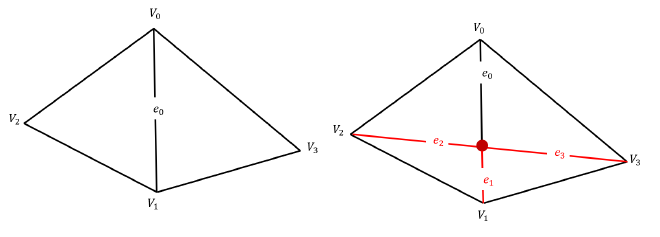
Part 5: Edge Split

#

The edge split operation is more complex than an edge flip. When splitting an edge, we insert a new vertex at its midpoint, introduce three new edges, two new faces, and six new halfedges, as illustrated in the figure. This operation involves significantly more pointer manipulations, requiring careful handling.

Unlike an edge flip, an edge split can be performed on a boundary edge. I implemented support for splitting boundary edges as well, which will be elaborated below. EXTRA CREDIT

Implementation Details

#

1. Identifying Key Elements. The process of identifying key elements follows a similar approach to the previous section. See the figure for a visual representation of the elements involved in the edge split.

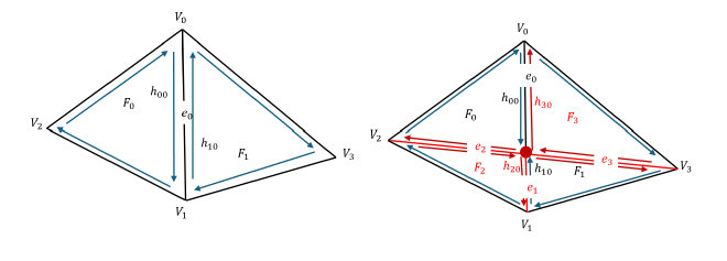
2. Creating the New Elements. The new elements introduced during the edge split include:

• A new vertex at the midpoint of the edge.
• A new edge \( e_1 \).
• Two new halfedges \( h_{20} \) and \( h_{30} \). Even if the original edge \( e_0 \) being split lies on a boundary, these elements must still be created.

3. Handling Each Side Separately. We determine whether \( F_0 \) and \( F_1 \) are boundary faces. The handling differs in the two cases, use \(F_0\) as an example:

• If \( F_0 \) is an interior face, a new edge \( e_2 \) is introduced to divide the two new triangles, following the labeled structure in the figure.
• If \( F_0 \) is a boundary face, the situation is different. Consider halfedges \( h_{00} \) and \( h_{20} \): since no new edge \( e_2 \) is created to separate them into two different triangles, they remain in the same face. In this case, their next pointers must be carefully updated: $$ h_{00} \rightarrow \text{next} = h_{20}, \quad h_{20} \rightarrow \text{next} = h_{00} \text{’s original next} $$

This careful pointer reassignment ensures that both boundary and non-boundary edges can be split correctly, maintaining proper manifold structure.

Result Gallery

#

The images below illustrate the edge split operation on a mesh with selected edges. The original mesh is shown on the left, while the split mesh is displayed on the middle, and right one shows the mesh after both split and flip.

Blow shows the result of splitting a boundary edge, the left one is the original mesh, and the right one is the mesh after splitting the boundary edge.

Left: Original; Right: Split Boundary Edge

---

Part 6: Mesh Subdivision

#

To perform mesh subdivision, we must apply a series of edge splits to generate a denser mesh with more faces. Additionally, specific adjustments are required to ensure that the new vertices, edges, and faces are well-distributed after subdivision.

Implementation Details

#

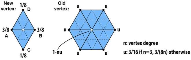
1. Compute New Positions for Existing Vertices. Each existing vertex updates its position based on the surrounding vertices’ locations. A common smoothing scheme, such as Loop subdivision, updates a vertex \( v_i \) as follows:

$$ v_i’ = (1 - n u) v_i + u \sum_{j=1}^{n} v_j $$

where:

• \( v_i \) is the original vertex position.
• \( v_j \) are the \( n \) neighboring vertices.
• \( u = \frac{3}{16}\) if \(n=3\), otherwise \(u = \frac{3}{8n}\). It is the weight factor.

Since the neighboring vertex positions are based on the original mesh, we store the updated positions separately before modifying the mesh.

2. Compute New Positions for Edge-Split Vertices. Each new vertex created from an edge split is positioned based on its two endpoint vertices and their neighboring vertices. The updated position for a new vertex \( v_e \) on edge \( (v_1, v_2) \) is: $$ v_e’ = \frac{3}{8} (v_1 + v_2) + \frac{1}{8} (v_3 + v_4) $$

where:

• \( v_1, v_2 \) are the endpoints of the edge being split.
• \( v_3, v_4 \) are the opposite vertices in the adjacent triangles sharing the edge.

3. Split Every Edge in the Mesh. We traverse all edges and apply the edge split operation. However, certain edges must be skipped:

• If the edge was created during the previous step (e.g., \( e_2, e_3 \) from the previous section), it should not be split in this iteration, skipping it.
• Although \( e_1 \) is also a newly created edge, it represents the same logical edge as \( e_0 \) (pre-split edge), so it should not be split either. To determine whether this kind of edge should be skipped: if an edge is not newly created and has one old vertex and one new vertex, it corresponds to \( e_1 \) and should be skipped.

4. Flip Any New Edge Connecting an Old and New Vertex. We traverse all edges again and check if an edge is newly created (e.g., \( e_2, e_3 \)). If is a new edge and has one old vertex and one new vertex, we perform an edge flip to improve mesh quality and maintain uniformity.

5. Update All Vertex Positions. Finally, we apply the previously computed new vertex positions to update all vertices in the mesh.

This sequence of operations ensures a well-distributed, subdivided mesh while maintaining smoothness and structure.

Subdivision Analysis

#

General Behavior

#

After applying Loop Subdivision, the mesh becomes smoother and more refined. The number of faces increases significantly, leading to a denser mesh with improved visual quality. Here are some examples of the subdivision process:

Effect on Sharp Corners and Edges

#

Loop subdivision tends to smooth too much to edges and corners, and causing huge movement of vertices. This can be seen in the following example:

For the teapot, the edge of the lid is smoothed out after subdivision, the sharp edge of the lid is no longer visible after subdivision. And the second example shows more significant movement of vertices, they are moved towards the center of the mesh.

There are two reason: The neighbors of the vertices on the sharp edges are far away from it; The degree of the vertices on the sharp edges is low.

1. For vertex on sharp edge, like those in second example, the neighbors are kind far away from it, the new position depends on the neighbors, so the vertex will move more than those with nearer neighbors.
2. If the degree of the vertex is low, according to the position update formula: $$ v_i’ = (1 - n u) v_i + u \sum_{j=1}^{n} v_j $$ where \(u=\frac{3}{8n}\), if \(n\) is not 3. If the degree \(n\) is low, \(u\) will be large, and the new position will be more affected by the neighbors, and thus the vertex will move more.

Thus to preserve sharp edges and corners, we can use pre-splitting to the edges that we want to keep sharp. As consequence, the vertices on the sharp edges and corners will have more near neighbors, and the new position will be more stable.

From the images above, we can see that the some sharp edges is preserved after subdivision, at least it doesn’t become a pure ring after subdivision.

Case Learning: Cube

#

After repeated subdivision, the cube becomes rounder and more spherical, with the sharp edges and corners gradually disappearing. And the cube also exhibits asymmetry.

Why Does the Cube Become Rounder? The rounding effect occurs because each vertex is repositioned based on its neighbors, same as discussed above, the neighbors are far away from the vertices, so the vertices will move more and become round.

Why Does the Cube Become Asymmetric? The asymmetry arises due to how triangles are arranged on each face of cube. They are not same at each face, when computing new vertex positions, each vertex uses a different set of neighbors in terms of both distance and relative position.

Mitigation Strategy. Pre-splitting some edges can introduce more near vertices, allowing better control over shape retention. Additionally, flipping edges to enforce a consistent triangular layout across faces.

Here are results, the triangle layouts are same on each face, and the cube is symmetric after subdivision. And it still has 6 faces, looks like a ‘smooth cube’ rather than a ‘ball’.