
Overview#
In this assignment, I implemented a basic rasterization pipeline, enabling the rendering of single-color triangles, colored triangles, and textured triangles on the screen. Below is a summary of the tasks completed:
- Task 1: Implemented basic single-color triangle rasterization. To improve performance, I implemented Tiled-Based Triangle Traversal, which accelerated the rendering process.
- Task 2: Implemented supersampling, significantly improving anti-aliasing. Additionally, I implemented Low-Discrepancy Sampling, which produced better rendering results for sharp triangle corners compared to grid-based sampling.
- Task 3: Implemented basic geometric transformations, including rotation, translation, and scaling. I also added a GUI feature that allows rotating the image around its center, regardless of its position on the screen, rotating the viewport.
- Task 4: Implemented Barycentric Coordinates, enabling color interpolation within triangles, allowing the rendering of smoothly rendered colored triangles.
- Task 5: Implemented basic texture mapping, comparing the effects of nearest sampling and bilinear sampling.
- Task 6: Implemented mipmap-based level sampling, which effectively reduced aliasing in most cases. Additionally, I implemented anisotropic filtering, which preserved fine details while maintaining good anti-aliasing performance. Using custom textures, I compared different sampling methods and mipmap level selection strategies to analyze their effects.
Task1: Drawing Single-Color Triangles#
Basic Process of Rasterization#
To render a triangle on the screen, we need to perform rasterization. The image or graphics to be displayed, such as the SVG file used here, are typically continuous in nature. Rasterization is the process of converting these continuous shapes into discrete, finite representations that can be written into the framebuffer, determining the color to be displayed at each pixel on screen.
The rasterization process basically is:
- Iterate all pixels that are possible in triangle;
- For each pixel, check if it is inside the triangle;
- If it is inside the triangle, fill the pixel with the color of the triangle.
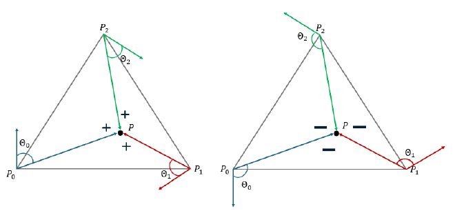
Given the coordinates of the three vertices of a triangle, we can derive the equations of its three edges. Given two vertices \(P_0=(x_0, y_0)\) and \(P_1=(x_1, y_1)\), and an arbitaty point \(P=(x, y)\), the equation of the line connecting them is given by: $$ \begin{aligned} L(x, y) = -(x-x_0)(y_1-y_0) + (y-y_0)(x_1-x_0) \end{aligned} $$
It can be also understood as the dot product of the vector \(V = (x-x_0, y-y_0)\) and the normal vector \(N = (y_1-y_0, x_0-x_1)\) of the edge, reflecting the angle \(\theta\) between the two vectors:
$$ V\cdot N = |V||N|\cos(\theta) $$
By substituting an arbitrary point’s coordinates \((x, y)\) into these equations, we can determine on which side of edge the point lies, according to the \(\theta\) is more than 90 or less. If we compute the edge equations in a consistent order (clockwise or counterclockwise) and evaluate the given point on all three edges, the point is inside the triangle if all results have the same sign (either all positive or all negative). It’s called the ‘point-in-triangle test’.
If thers is point lies on the line, I follow the convention of OpenGL: if the point lies on horizontal and top edge or non-horizontal and left edge, it is considered inside the triangle.
The simplest approach is to iterate over all pixels and check whether each one is inside the triangle using the above method. However, this approach is computationally expensive. A straightforward optimization is to compute the bounding box of the triangle and only iterate over pixels within this box.
Tiled Triangle Traversal#
Based on bounding box traversal, I adopt a more efficient approach: Tiled Triangle Traversal.
Overview#
In essence, the screen is divided into small square tiles, and each tile is frist tested to determine whether it is entirely inside or entirely outside the triangle. If a tile is fully inside the triangle, all its pixels can be directly filled without individual checks. If a tile is completely outside, it can be skipped entirely. For tiles that partially overlap with the triangle, each pixel within the tile is individually checked.
Tile Test#
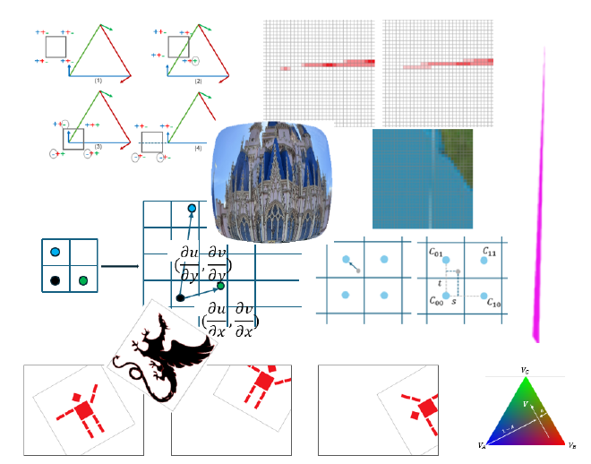
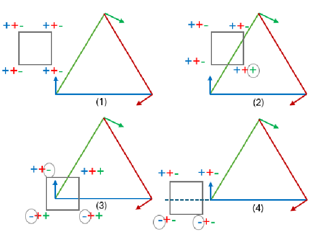
To check if a tile is fully inside or outside the triangle, use four corners of the tile \(P_1, P_2, P_3, P_4\) to do the ‘point-in-triangle test’, we can get 4 arrays of results, each has 3 elements, the sign of element is corresponding to which side the corner lies on the three edges. Each result array is denoted as: $$ S_k = \left[ \text{sign}(L_1(P_k)), \text{sign}(L_2(P_k)), \text{sign}(L_3(P_k)) \right] = \left[ s_{k1}, s_{k2}, s_{k3} \right] $$ Then \(s_{ij}\) is test result of corner \(i\) with regard to line \(j\). There will be three cases:
Fully Inside the Triangle. If all four points are inside the triangle, same as we discussed above, all the results should have the same sign, thus all \(s_{ij}\) are the same.
Fully Outside the Triangle. If all four corners lie on the same side of all three edges, then for each test regard to line j, all results for four corners are identical: \( s_{1j} = s_{2j} = s_{3j} = s_{4j}, \forall j \in {1,2,3} \)
Partially Inside the Triangle. All other cases are considered as partially inside the triangle.
This method is simple yet effective in detecting most cases of tiles being completely inside or completely outside the triangle. One fully outside case will be missed, when the tile is crossing the extension of one edge, shows in the figure below. But it is still a good trade-off between accuracy and efficiency.
Compare to bounding box#
EXTRA CREDIT: If we find out some tiles are fully inside or outside the triangle, all the pixels in the tiles can skip the ‘point-in-triangle test’, and save time. And the ‘Tile Test’ only cost time for four times of ‘point-in-triangle test’. Consider the worst case, none of tiles are fully inside or outside the triangle, all pixels need to be tested. Then the time complexity is still \(O(n_b)\), \(n_b\) is number of pixels in bounding box, which is same as bounding box traversal.
The choice of tile width significantly impacts the efficiency of the rasterization process. If a smaller tile width is chosen, more tiles will be entirely inside or outside the triangle, reducing computation time. However, if the width is too small—for example, the overhead of performing four point-in-triangle tests per tile will increase, making the process as slow as the original method, even if all tiles are outside the triangle. In the implementation, I selected a tile width of 16. The comparasion between bounding box traversal and tiled triangle traversal is shown in the table below.
| Render Time(ms) | Bounding Box Traversal | Tiled Triangle Traversal (w=16) |
|---|---|---|
| basic-3 | 32.58 | 24.67 |
| basic-4 | 1.99 | 1.71 |
| basic-5 | 5.72 | 4.93 |
| basic-6 | 3.11 | 2.88 |
Results Gallery#
The following image shows the rendering result of single-color triangles. As observed, without implementing any anti-aliasing techniques, jagged edges can be seen along the triangle boundaries.


Task2: Antialiasing by Supersampling#
Supersampling Overview#
As its name suggests, supersampling involves taking multiple samples per pixel instead of just one. The sampling rate represents the number of samples taken within a single pixel.
Why is Supersampling Helpful?#
A single pixel provides a coarse representation of a small area of the continuous-space triangle. In the previous Task 1, we determined whether a pixel inside a triangle by evaluating at a single point— the pixel center. If this point happened to be near the triangle’s edge, the pixel might be partially inside and partially outside the triangle. However, this approach treated it the same as fully inside pixels, filling it entirely with the triangle’s color, leading to jagged edges.
By sampling multiple points per pixel, some of the samples might fall outside the triangle, allowing us to process these pixels differently from fully covered ones, thus softening the triangle edges and achieving anti-aliasing effects.
Also according to the theory of signal processing, if we perform supersampling, it is increasing the sampling rate. That is to say Nyquist frequency is also increased, then we can sample higher frequency signals without aliasing artifacts.
Data Structure Adjustments#
The primary modification is increasing the length of the \lstinline|frame_buffer| by a factor of \(n\), the sampling rate. For a pixel at \((x, y)\), its corresponding samples are stored in the buffer region: $$ (y \times \text{width} + x) \times n \quad \text{to} \quad (y \times \text{width} + x) \times n + (n - 1) $$ After sampling, the final pixel color is obtained by averaging the colors of all \(n\) samples, effectively blending the colors at sub-pixel levels to reduce aliasing.
Detailed Implementation#
To implement supersampling, I used two different approaches: grid-based supersampling and low-discrepancy sampling. The possible sampling rates are \(n = 1, 4, 9, 16\), ensuring that \(\sqrt{n}\) is always an integer.


Grid-Based Supersampling#
This method performs sampling on a higher-resolution grid. Each original pixel is subdivided into \(\sqrt{n} \times \sqrt{n}\) sub-pixels, and the center position of each sub-pixel is tested using the point-in-triangle test. If the sub-pixel is inside the triangle, it is assigned the triangle’s color. Finally, as discussed earlier, the final pixel color is computed by averaging the colors of its \(n\) samples.
Low-Discrepancy Sampling#
EXTRA CREDIT: In grid-based sampling, the center position \((0.5w, 0.5w)\) of each sub-pixel is used for testing, where \(w\) is the width of a sub-pixel. Instead of using fixed center positions, low-discrepancy sampling chooses sampling points using two random values \((r_1 w, r_2 w)\), where \(r_1\) and \(r_2\) are low-discrepancy numbers ensuring a more uniform distribution.
I used the Halton sequence, choosing base 2 for \(r_1\) and base 3 for \(r_2\). For the \(i\)-th supersampling point, the corresponding values are taken from the \(i\)-th element of the sequence. This method ensures better coverage of the pixel area, leading to a more accurate approximation of anti-aliasing effects. See results gallery for comparison, the low-discrepancy has better anti-aliasing effect on the edge of triangle. It’s more obvious when sample rate is not that high.
I also implemented a simple version that \(r_1\) and \(r_2\) are generated randomly, the results are much worse than Halton sequence.
Results Gallery#
The following images show the rendering results of supersampling with different sampling rates and methods. The first row shows the results of grid-based supersampling, while the second row shows the results of low-discrepancy sampling. And last row shows the results of random sampling. The images are displayed in the order of increasing sampling rates(1, 4, 16).


When sampling rate is 4, the skinny corner of red triangle is more smooth in low-discrepancy sampling than grid-based sampling, where the grid-based one still have some isolate pixels. When sampling rate is 16, the difference is not that obvious.


Task3: Transforms#
Play with Cubeman#
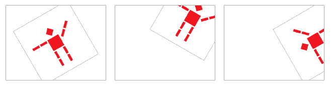
This section implements basic transformations, including rotation, translation, and scaling. I created a new Cubeman, attempting to walk with synchronized arm and leg movements.
Specifically, I rotated the shoulder block by -45 degrees and the right leg by -90 degrees. However, the entire right arm and right leg rotated together, demonstrating the characteristics of hierarchical transforms.


Rotate Viewport#
EXTRA CREDIT: In this section, I implemented a new GUI feature that allows the viewport to rotate using the Q and E keys. The rotation is performed around the center of the SVG image, regardless of its position on the screen.
The implementation requires consideration of three coordinate systems: 1) SVG coordinate system; 2) Normalized Device Coordinates coordinate system; 3) Screen coordinate system. To ensure that the image rotates around its center in screen space, it must also rotate around its center in NDC space. The process is as follows: First, we retrieve the width and height of the SVG image to determine its center coordinates. Using the svg_to_ndc transformation matrix \(m\), we transform the image center from SVG space to NDC space. We then construct three transformation matrices:
- Translation \(T\): Moves the center to the NDC origin (0,0);
- Rotation \(R\): Performs the desired rotation;
- Inverse Translation \(T_{\text{inv}}\): Moves the center back to its original position;
Combining these transformations, the updated
svg_to_ndcmatrix is given by:
$$ m’ = T_{\text{inv}} \cdot R \cdot T \cdot m $$
Task4: Barycentric Coordinates#
During the rendering process, various forms of interpolation are involved, particularly for interpolating values inside a triangle. Given a triangle with three vertices, we can interpolate values such as texture coordinates or color for any point inside the triangle. Barycentric coordinates provide an elegant way to achieve this.
For any point \(V\) inside the triangle defined by vertices \(V_A, V_B, V_C\), its coordinates can be expressed as:
$$ V = \alpha V_A + \beta V_B + \gamma V_C $$
By substituting \(V_A, V_B, V_C\) with the desired values (such as color, UV coordinates…), we can compute the interpolated value at \(V\).
Taking \(\alpha\) as an example, it represents the ratio between the distance from point \(V\) to edge \((V_B, V_C)\) and the distance from vertex \(V_A\) to the same edge. Using the previously discussed line equation, we can derive the equation for the line passing through \(V_B\) and \(V_C\):
$$ L(x, y) = -(x - x_B)(y_C - y_B) + (y - y_B)(x_C - x_B) $$
By substituting the coordinates of \(V_A\) and \(V\) into this equation, we obtain:
$$ \alpha = \frac{L(x_V, y_V)}{L(x_A, y_A)} $$
While this equation does not directly represent a physical distance, the value of the line equation is proportional to the distance. Since we only need the ratio, we can use this formulation directly.

Furthermore, the barycentric coordinates \(\alpha, \beta, \gamma\) can also be interpreted as the relative areas of the three sub-triangles formed by \(V\) within the original triangle.

result test-7
Task5: “Pixel sampling” for texture mapping#
Texture Mapping Overview#
Using the Barycentric Coordinates implemented in the previous task, if the UV coordinates of the three triangle vertices (which define their positions in texture space) are known, we can easily determine the UV coordinates for any point inside the triangle.
However, this introduces the same issue as in Task 1: textures are discrete images composed of individual pixels, but the computed UV coordinates represent continuous locations in texture space. The challenge is determining which pixel’s color should be assigned to a given point.
Nearest Sampling#
The simplest approach is nearest-neighbor sampling:
- Compute the UV coordinates of the point;
- Round the coordinates to the nearest integer pixel position;
- Assign the color of the corresponding texture pixel to the point.
But there will be an issue: Texture Magnification. If the target triangle is large, but the texture resolution is low, many points in the triangle might map to the same texture pixel. This results in visible blocky artifacts in the final image, where multiple screen pixels share the same color, forming some noticeable square regions.
Bilinear Sampling#
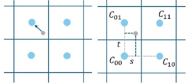
To mitigate the blocky artifacts caused by nearest sampling, bilinear interpolation can be used. Instead of selecting a single nearest pixel, this method computes a weighted average of the four nearest pixels, leading to a smoother appearance.
Once the UV coordinates are computed, determine the four nearest texture pixels. And then define two interpolation parameters:
- \(s\): The horizontal fractional distance from the left pixel center.
- \(t\): The vertical fractional distance from the lower pixel center.
Using these parameters, the final color is computed using a bilinear interpolation formula: $$ C = (1 - s)(1 - t) C_{00} + s(1 - t) C_{10} + (1 - s)t C_{01} + st C_{11} $$
where \(C_{00}, C_{10}, C_{01}, C_{11}\) are the colors of the four surrounding texture pixels.
By blending the four nearest texture colors, bilinear sampling ensures smooth transitions between adjacent texture pixels. Even if multiple points map to the same texture pixel, their colors will still vary based on their relative positions, preventing blocky artifacts in the final image.
Results Gallery#
The following images show the rendering results of texture mapping using nearest and bilinear sampling. The first row shows the results of nearest sampling, while the second row shows the results of bilinear sampling. First column is sampled with sample rate 1, second column is sampled with sample rate 16.


When the sampling rate is low, the difference between nearest sampling and bilinear sampling becomes more pronounced, especially in stretched areas of the image, such as the Pixel Inspector display region.
Since the image is stretched, the triangle areas increase, but the texture resolution remains the same. As a result, more points in the rendered triangle map to the same texture pixel.
Task6: “Level samping” with mipmaps for texture mapping#
Level Sampling Overview#
In the previous task, we discussed techniques to address texture magnification. However, when a small triangle covers a large texture area, a single screen pixel may map to multiple texture pixels, leading to texture minification. To solve this issue, mipmaps and level sampling are used.
A mipmap is a sequence of precomputed downsampled versions of the original texture, ranging from full resolution to progressively smaller versions downsampled by factors of 2. Using a lower-resolution texture allows points that originally covered multiple texture pixels to instead map to a single pixel in a lower-resolution texture, reducing aliasing.
The appropriate mipmap level \(D\) is determined as follows:
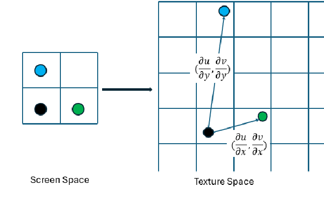
$$ D = \log_2 \max \left( \sqrt{\left( \frac{\partial u}{\partial x} \right)^2 + \left( \frac{\partial u}{\partial y} \right)^2}, \sqrt{\left( \frac{\partial v}{\partial x} \right)^2 + \left( \frac{\partial v}{\partial y} \right)^2} \right) $$
This equation measures the rate of change of texture coordinates \((u, v)\) with respect to screen-space coordinates \((x, y)\). A large \(D\) value indicates that a small change in \(x\) or \(y\) results in a significant transformation in \(u\) and \(v\), requiring a higher downsampling level to prevent aliasing. Typically, \(D = 0\) means using the original texture, while \(D = n\) means using a texture downsampled by \(n\) times.
Since the computed \(D\) is usually not an integer, two methods are used for selecting the appropriate mipmap level. Nearest D simply rounds \(D\) to the nearest integer level, but this can cause abrupt transitions in texture quality, leading to visible seams or blocky changes in regions where \(D\) varies rapidly. A better approach is linear interpolation, where we sample from two adjacent mipmap levels and blend the results. Given \(D\), we define \(D_{\text{low}} = \lfloor D \rfloor\) and \(D_{\text{high}} = \lceil D \rceil\), then compute an interpolation weight \(t = D - \lfloor D \rfloor\) to blend the two levels:
$$ C = (1 - t) C_{\text{low}} + t C_{\text{high}} $$
This ensures a smooth transition between mipmap levels, reducing visual artifacts caused by abrupt level changes. By combining mipmaps with interpolated level sampling, texture minification artifacts are minimized, leading to a more consistent rendering quality.
Anisotropic Filtering#
EXTRA CREDIT: Mipmap downsampling is performed simultaneously in both the \(x\)- and \(y\)-directions, which can lead to issues in certain cases. As illustrated in the figure, when texture coordinates \((u, v)\) change rapidly along the \(y\)-axis but slowly along the \(x\)-axis, the previous formula for computing \(D\) simply takes the maximum value. This results in a higher downsampling level to accommodate the rapid changes along \(y\), but since the texture is reduced in both directions, details that could have been preserved in the \(x\)-direction are lost, making the texture appear excessively blurred in some areas.
To address this issue, anisotropic filtering can be used. Many implementations use ripmap to handle this, but to avoid modifying the existing framework, I chose an alternative method.
The key idea is to analyze the rate of texture coordinate changes in different directions. The vectors \(G_x =(\partial u / \partial x, \partial v / \partial x)\) and \(G_y =(\partial u / \partial y, \partial v / \partial y)\) represent the primary directions of texture variation. The vector with the larger magnitude indicates the direction where UV coordinates change the most. By computing the ratio of the larger magnitude to the smaller one, we can determine whether the texture varies significantly more in one direction than the other. If this ratio is large, it suggests that mipmapping alone is insufficient. It can be calculated as: $$ |G_x| = \sqrt{\left( \frac{\partial u}{\partial x} \right)^2 + \left( \frac{\partial v}{\partial x} \right)^2}, \quad |G_y| = \sqrt{\left( \frac{\partial u}{\partial y} \right)^2 + \left( \frac{\partial v}{\partial y} \right)^2} $$
$$ N = \frac{\max(|G_x|, |G_y|)}{\min(|G_x|, |G_y|)} $$
To correct this, for a given point with texture coordinates \((u, v)\), its primary variation direction \(d\), and the anisotropy ratio \(N\), I perform additional sampling along the dominant direction. Specifically, I sample at \((u, v) + 1d\), \((u, v) + 2d\), …, \((u, v) + Nd\) and compute the average of these sampled values to obtain the final color.

Sample more points along the dominant direction
Since the standard mipmap approach would already downsample too much in the slower-changing direction, I adjust the sampling at the \(D-1\) level instead of directly using \(D\), helping to retain more texture details.
UPDATE: The more proper way to do this is, use \(D = \log_2 \min(|G_x|, |G_y|)\).
Comparison of Different Sampling Methods#
The following images show the rendering results of texture mapping using different sampling methods.
Discussion on Anti-Aliasing Effects#
Nearest sampling consistently produces blocky patterns, making it the least effective method in terms of anti-aliasing. Bilinear sampling generally provides good results in most cases. When mipmaps are used, sharp aliasing artifacts are significantly reduced, but the overall image tends to become blurry, especially in trilinear sampling.
By analyzing the Pixel Inspector view of the castle corner, it is evident that anisotropic filtering implemented with my simple approach achieves anti-aliasing quality comparable to bilinear sampling while retaining sharper details when using mipmaps. For example, the right edge of the castle appears much clearer compared to standard trilinear sampling.
Comparison of Time Complexity#
In terms of computational cost, all interpolation-based methods are slower than nearest sampling, and the more interpolation involved, the slower the process. From the perspective of sampling methods, the complexity follows:
$$ \text{Nearest} < \text{Bilinear} < \text{Anisotropic Filtering} $$
Regarding mipmap usage, the hierarchy of complexity is:
$$ \text{All Zero} < \text{Nearest} < \text{Linear} $$
This suggests that while anisotropic filtering is computationally more expensive than bilinear sampling, it provides a improvement in texture clarity while maintaining effective anti-aliasing.